| Neural networks provide a rather different
approach to reasoning and learning. A neural network consists
of many simple processing units (or neurons) connected together.
The behaviour of each neuron is very simple, but together a collection
of neurons can have sophisticated behaviour and be used for complex
tasks. There are many kinds of neural network, so this discussion
will be limited to perceptrons, including multilayer perceptrons.
In such networks the behaviour of a network depends on weights
on the connections between neurons. These weights can be learned
given example data. In this respect, neural networks can be viewed
as just another approach to inductive learning problems.
Neural networks are often described as using a sub symbolic representation
of expert knowledge. There is no meaningful symbol structure (e.g.,
rule or decision tree) produced that can easily be interpreted
by an expert, but a collection of simple units that, by the way
they are connected and weighted, combine to produce the overall
expert behaviour of the system. This means that it is hard to
check that the learned knowledge is sensible. To a large degree
it has to be treated as a "black box" which, given some
inputs, returns some outputs.
Neural networks are biologically inspired, so this section will
start with a brief discussion of neurons in the human brain.
Biological Neurons
The human brain consists of approximately ten thousand million
simple processing units called neurons. Each neuron is connection
to many thousand other neurons. The detailed operation of a neuron
is complicated and still not fully understood, but the basic idea
is that a neuron receives inputs from its neighbors, and if enough
inputs are received at the same time that neuron will be excited
or activated and fire. giving an output that will be received
by further neurons.
Figure 7.5 illustrates the basic features of a neuron. The soma
is the body of the neuron, dendrites are filaments that provide
inputs to the cell, the axon sends output signals, and a synapse
(or synaptic junction) is a special connection which can be strengthened
or weakened to allow more or less of a signal through. De-pending
on the signals received from all its inputs, a neuron can be in
either an excited or inhibited state. If excited, it will pass
on that "excitation" through its axon, and may in turn
excite neighbouring cells.
The behaviour of a network depends on the strengths of the connections
be-tween neurons. In the biological neuron this is determined
at the synapse. The synapse works by releasing special chemicals
called neurotransmitters when it gets an input. More or less of
such chemicals may be released, and this quantity may be adjusted
over time. This can be thought of as a simple learning process.
The Simple Perceptron:
A Basic Computational Neuron
A simple computational neuron based on the above can be easily
implemented. It just takes a number of inputs (corresponding to
the signals from neighbouring cells), adjusts these using a weight
to represent the strength of connections at the synapses, sums
these, and
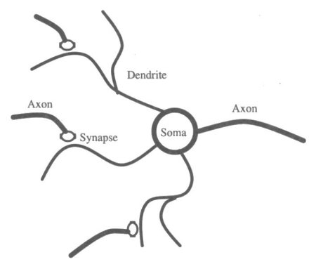
Figure 7.5 Basic Features of a Biological
Neuron.
fires if this sum exceeds some threshold.
A neuron which fires will have an output value of 1, and otherwise
output 0. More precisely, if there are n inputs (and n associated
weights) the neuron finds the weighted sum of the inputs, and
outputs 1 if this exceeds a threshold t and 0 otherwise. If the
inputs are X1…Wn, with weights W1…Wn :
If W1X1 + … + WnXn > t
then output = 1
else output = 0
This basic neuron is referred to as a simple
perceptron. and is illustrated in Figure 7.6. The name "perceptron"
was proposed by Frank Rosenblatt in 1962. He pioneered the simulation
of neural networks on computers.
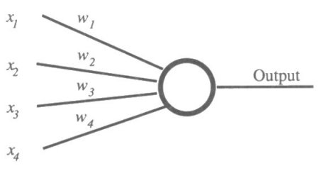
Figure 7.6 Basic Computational Neuron.
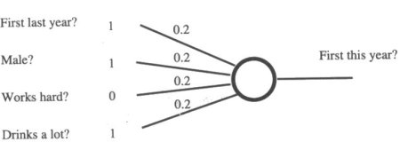
Figure 7.7 Neuron with Example Inputs and
Weights.
A serious neural network application would
require a network of hundreds or thousands of neurons. However,
it is possible to achieve learning even with a single isolated
neuron. Learning, in neural networks, involves using example data
to adjust the weights in a network. Each example will have specified
input-output values. These examples are considered one by one,
and weights adjusted by a small amount if the current network
gives the incorrect output. The way this is done is to increase
the weights on active connections if the actual output of the
network is 0 but the target output (from the example data) is
1, and decrease the weights if the actual output is 1 and the
target is 0. The whole set of examples has to be considered again
and again until eventually (we hope) the network converges to
give the right results for all the given examples.
This will be illustrated using an example before stating the learning
algorithm more precisely. Our student example can be used. Each
feature (works hard etc.) can be represented by an input. so x1
= 1 if the student in question got a first last year, x2 = 1 if
they are male, and so on. The output corresponds to whether they
end up getting a first, so output = 1 if the student gets a first.
Initially the weights are set to some small random values, but
to simplify the example we'll assume each weight has the value
0.2. The value of the threshold t also needs to be decided, and
we'll make it be 0.5. The amount that the weights are adjusted
each time will be called d, and for this example will have the
value 0.05.
Figure 7.7 illustrates this, with example data from the first
student example (Richard). Before any learning has taken place
the output of this network is 1, as the weighted sum of the inputs
is 0.2 + 0.2 + 0.2 = 0.6, which is higher than the threshold of
0.5. But Richard didn't get a first! So all the weights on active
connections (those with inputs of 1) should be decremented by
0.05. The new weights will be 0.15, 0.15, 0.2 and 0.15.
The next example (Alan) is now considered. His inputs are 1, 1,
1 and 0. The current network gives an output of 0 (the weighted
sum is exactly 0.5), but the correct output is 1, so the relevant
weights are incremented by d, to give new weights of 0.2, 0.2,
0.25, 0.15. Note how the weight for "works hard" is
now higher than the others, while "drinks a lot" is
lower: Alan and Richard are pretty similar in many ways, only
Alan works harder than Richard and doesn't drink.
All the other examples are considered in the same way. No adjustments
to the weights in the network are needed for Alison, Jeff or Gail.
However, after Simon is considered the weights are adjusted to
give 0.2, 0.15, 0.2 and 0.1.
Learning doesn't end there. All the examples must be considered
again and again until the network gives the right result for as
many examples as possible (the error is minimized). After a second
run-through with our example data the new weights are 0.25, 0.1,
0.2 and 0.1. These weights in fact work perfectly for all the
examples, so after the third run-through the process halts. Weights
have now been learned such that the perceptron gives the correct
output for each of the examples.
If a new student is encountered then to predict their results
we use the learned weights. Maybe Tim got a first last year, works
hard, is male, but drinks. We would predict that he will get a
first.
In this example we can ascribe some meaning to the weights: getting
a first last year and working hard are both positive (particularly
getting a first), while being male or drinking are less important,
with maybe a slightly negative impact. However, for more complex
networks it becomes extremely hard to make any sense of the weights;
all we know is whether the network gives the right behaviour for
the examples.
Anyway, the basic algorithm for all this is as follows:
o Randomly initialize the weights.
o Repeat
- For each example
* If the actual output is 1 and the target
output is 0, decrement the weights on active connections by d;
* If the actual output is 0 and the target output is 1, increment
the weights on active connections by d;
until the network gives the correct outputs
(or some time limit is exceeded).
Now, although this algorithm worked fine
for the student problem, there are some sets of examples where
there is just no set of weights that will give the right behaviour.
A famous example is the exclusive or function, which is meant
to output a 1 if one input is I and the other is 0, and a 0 otherwise.
It's just not possible to find a set of weights for a simple perceptron
to implement this function. Minsky and Papert, in their book Perceptrons,
showed formally in 1969 just what func-tions simple perceptrons
could and couldn't represent. This critique was one of the causes
of a decrease of interest in neural networks in the 1970s. Only
relatively recently has interest been revived, with more complex
versions of the perceptron proposed which don't have the same
fundamental limitations. The next section will just briefly sketch
a widely used approach.
More Complex Networks and Learning
Methods
So far we've just considered what can be done with a single neuron,
using the sim-plest possible method for calculating the output
and for learning. This works for some simple examples and illustrates
the general idea, but for more complex prob-lems we need to go
back to the idea of having an interconnected network of neurons
(or units). These are arranged in layers, with outputs from one
layer feeding into inputs in the next layer. We'll consider multilayerperceptrons.
Figure 7.8 illustrates a possible (but very small) network with
three layers of neurons. This network has an input layer, a hidden
layer and an output layer. Each neuron may be connected to several
in the next layer (copying its output to the inputs of these units).
The input layer does no more than distribute the input values
to the next layer and sometimes such a network is referred to
as a two-layer network, as the input layer isn't counted. The
output layer may consist of several units. This means that the
network can calculate (and learn) things where there are several
possible answers, rather than just a yes/no decision (maybe distinct
units would be used for the results "first", "2-1",
"2-2" and "third").
It is possible to have such a network where each unit corresponds
to a simple perceptron as described in the previous section. Given
some inputs the outputs of the first layer of units would be calculated
as before, and these outputs used as the input values for the
next layer of units. However, it turns out that if the old rule
for calculating the output of a unit is used then there is no
good learning method that can be applied. There is no problem
with adjusting the weights in the last layer (feeding into the
output units); this could be done exactly as before. But it is
unclear how the weights between the input and hidden layer should
be adjusted. More complex networks may have more than one hidden
layer, and here the weights between hidden layers must somehow
be obtained.
The back propagation rule, proposed in 1986 by Rumelh art, McClelland
and
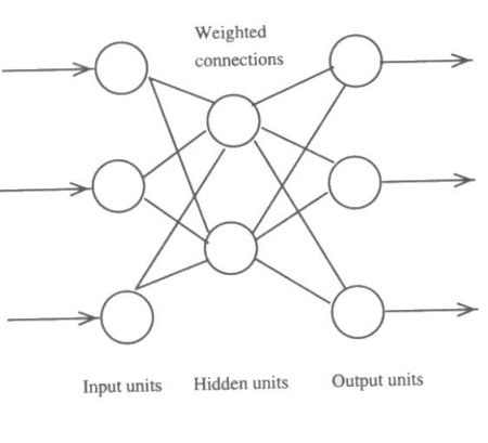
Figure 7.8 A Small Multllayer Network.
Williams, specifies how this can be done.
The method is substantially more complex than simple perceptron
learning, so will not be described fully here; more details are
given in the further reading at the end of the chapter. However,
the general idea involves first using a slightly more complex
function to determine the activation state (and hence output)
of a unit. This function, rather than just giving a value of 0
or 1, gives a value between 0 and 1. This means that it is possible
to get an idea from the output just how far off the unit is from
giving the right answer. In turn, this means that weights can
be adjusted more if the output is completely wrong than if the
output is almost right. The amount adjusted depends on the error
term which is just the difference between the target and actual
output. This error term can be calculated directly for the final
layer of weights, but to adjust weights in earlier layers it has
to be back propagated to earlier layers. The error term for units
in such layers is calculated by taking a weighted sum of the error
terms of the units that it is connected to.
Neural Network Applications
Neural nets are now being (fairly) widely used in practical applications,
so it's worth talking briefly about how a neural net application
might be developed. This discussion will assume that the back propagation
learning rule is to be used in a multilayer network. Many other
kinds of network and learning methods are possible.
Generally the method can be used whenever we have a lot of training
data, and want to produce a system that will give the right outputs
for the given inputs in the data. With luck (and judgement) the
system will also give sensible outputs for new input combinations
which don't exist in the training data.
Although it is possible to use neural networks for many sorts
of problems they tend to be particularly useful for pattern recognition
tasks, such as character recognition. As a simple example of
this, suppose we have lots of data corresponding to the digits
0-9 in various different fonts (e.g., 9, 9, and 9). For each we
have a small bitmap corresponding to the digit, and data on which
digit it is. We want a system that, given a bitmap image, can
recognize which digit it is. One way to set up a neural net for
this problem is to have an input unit for each pixel in the bitmap,
and an output unit for each digit of interest. (For a given digit
we'd require that only the relevant output was activated.) One
or more hidden layers could be used between these two. After training
with all the example data it should work for new fonts not yet
encountered.
To test the trained network it is really necessary to reserve
some of the training data to use for testing. So, initially the
data available might be split-in-two into training and test data.
The network would be trained using the training data, and then
tested with the remainder. If it gave good results for the test
data (not used in training) this suggests that it will also give
good results for new problems (e.g., fonts) for which data is
not yet available.
This example application is one where it
would be quite hard to write a conventional rule-based system
for determining which digit it was, or even to induce a decision
tree based on the data, yet humans find it quite easy to recognize characters by visual inspection. Neural networks seem to be good
at tasks like this which involve finding patterns in visual or
auditory data. Other related applications of neural networks
include: learning to pronounce English words; learning to distinguish
tanks from rocks in military images; learning to recognize people's
handwriting; learning to determine whether someone has had a heart
attack given their ECG signal.
Neural networks can also be applied to other kinds of learning
problem. One example application is determining whether to give
people credit given data on characteristics (e.g., home-owner?)
and current creditworthiness. For some of these problems more
conventional learning methods (such as ID3, and other statistical
methods) can and have been used just as successfully. The methods
can be compared by using training and test data as mentioned above
and finding out which does best on the test data. However, often
what is found is that there isn't that much difference between
the results of the different methods, and the results depends
more on the example data available and the features chosen than
the method used in learning!
Although there are simple commercial neural network tools available
that appear as easy to use as a spreadsheet, making best use
of the technique requires some understanding of the underlying
algorithms. For serious neural network development it is important
to consider carefully how to map features of the problem to input/output
nodes, what (if any) hidden layers to have in between, what learning
method to use, and how to set parameters (such as d and t above).
There are no simple rules for all this, so both study and experience
is needed. Unfortunately the algorithms involved are fairly mathematical,
so making best use of neural net software still requires some
mathematical competence.
Comparing Learning Methods
This chapter has introduced a range of different methods that
can be used in learning a general rule or concept from some example
data, using a single problem to illustrate each method. There
are many other learning methods that could be discussed, and
many statistical methods that can also be applied.
The different methods can be compared in
many ways. We'll just focus on two: the complexity of the knowledge
that can be learned, and how well the method can handle noisy
data.
Each method can learn to classify "concepts" (e.g.,
students, diseases, digits) given their features. Some of the
methods can learn more complex associations
between features and category4. Neural networks,
in particular, can in principle learn an arbitrarily complex function
associating inputs and outputs, while version space learning only
works well for simple rules involving conjunctions of facts. Decision
trees are somewhere in between. Genetic algorithms can be applied
to a variety of different concept representations - one can imagine
them being used where concepts were represented as decision trees,
and the crossover operation involved swapping tree fragments -
but do require that parts of a potential solution can be combined
in a sensible way.
Some of the methods require that the data contains no oddities
or exceptions to the rule that we want to learn. Imagine that
we have data on a thousand students. For nine hundred and ninety-nine
of them, the rule that "if you work hard and did well last
year you'll do well this year" works just fine. But there
is one odd one out who has somehow failed this year for whatever
reason. Such data is referred to as noisy. For most applications
we'd still want to learn the rule which works for the vast majority.
Yet, in their basic form, many methods would fail to find a solution.
Although there is not space to discuss in detail how the methods
can be adapted to work, it is easy to see roughly how things might
work. It is very hard to adapt version space search for noisy
data, but decision tree induction can be adapted if we relax the
criterion that a leaf node in the tree must contain examples all
of the same result category. We could, for example, mark the node
as "Gets a first" even if only 90% of the example students
with the given features did. Genetic algorithms can be moderately
easily adapted if we give up when we have a sufficiently high
(if not perfect) score. Neural networks work well without adaptation.
Although neural networks appear to be winning at this point, at
least if we want to learn complex rules given noisy data, they
have one clear disadvantage. Neural networks are opaque: it is
hard to check that the weights correspond to something sensible.
Although there are methods being developed to obtain explanations
of a neural network's decisions, and to convert neural networks
into a more inspectable format, these methods are not yet well
developed.
So. although the use of neural networks is in many ways the most
powerful method described, it may not always be the most appropriate
one. It is, in essence, a complex mathematical technique for producing
a classification system from ex-ample data. Other methods can
be used, with decision tree induction a particularly appropriate
one where a simple and understandable resultant system is required.
Other statistical methods should also not be ignored, although
not discussed in this book.
For a particular problem or application, the performance of different
approaches may be compared using training and test data for that
problem. However, for a prac-tical application what is often key
is the quality of the data. If you completely forgot to ask the
students what grade they got last year then that fact would be
unavailable to the learning program and NO algorithm could do
very well. Similarly, if you only had a small set of atypical
example students (maybe a group of friends, who are likely to
have features in common) then the resultant system, whatever learning
algorithm is used, would not do well given new test data. So it
is critical to have a large and representative sample for the
examples, and good predictive features. To some extent good features
may be discovered by consulting experts in a given field (e.g.,
asking what symptoms are important for distinguishing diseases).
There are also statistical methods that can be used to help determine
these. So to make the best use of machine learning methods it
may be useful to know some statistics.
Some methods may do well on some problems
but very badly on others. So that different methods can be compared
across a whole range of problems, large example datasets have
been made publicly available. If a new learning method is developed
it can be tested on some or all of these to see if it does better
on these problems.
Summary
- Machine learning techniques can be used
to automatically produce systems for doing certain classification
tasks, given examples of cases that have been correctly classified
by experts.
- Machine learning can be viewed as involving
a search for a rule fitting the data. Version space learning provides
a way of managing this search process. Genetic algorithms can
be used when the search space would be too big. Genetic algorithms
work by combining two moderately good possible solutions to (hopefully)
obtain a better "child" solution.
- The learning methods vary in the complexity
of the rule that can be learned. Version space learning, for example,
cannot easily be used to learn rules in-volving disjunctions.
Neural networks can in principle learn arbitrary functions.
- Decision tree induction is a widely used
method that produces the simplest decision tree that will correctly
classify the training data. The best input feature for splitting
examples into different categories is found, and the algorithm
called recursively.
- Neural networks learn by repeatedly adjusting
weights on links between nodes, until the correct output is given
for all the training examples.
- In practice the quality of results may
depend more on the training data than the learning method chosen.
|